Description
Problem 1. (computer) (5 points)
Write a program to perform a Metropolis Monte Carlo simulation of the 2D Ising model
in zero field (H = 0) and on a square L×L lattice. The Hamiltonian of this model is given
by
H = −J ∑
hi, ji
sisj (si, j = ±1)
where the sum is over all distinct nearest-neigbor pairs and si and sj are the values of the
spins at the lattice sites i and j. Set J = 1. Use periodic boundary conditions and spin-flip
updates. Temperatures are expressed in energy units. Time is expressed in units of Monte
Carlo steps (MCS) (1 MCS = 1 update per spin on average, i.e. total of L × L random
updates).
(a) Check that the ground state energy is calculated correctly. (Use all-spins-up or allspins-down as your initial configuration and calculate the energy of this configuration.)
For the following, the task is to study the 32×32 Ising model at three different temperatures: T = 2.1, 2.265 and 3.5. Note: the middle temperature T = 2.265 is difficult and
the results will look different than for the other two cases.
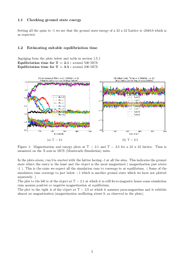
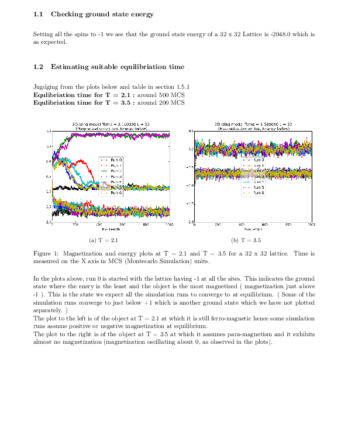
(b) Estimate a suitable equilibration time for T = 2.1 and 3.5. Perform several short runs
and plot the magnetization m and the internal energy u per spin as a function of time (in
MCS). Use a random spin configuration as your initial state. Remember to use different
random number sequences for the separate runs.
(c) For T = 2.265, perform a long simulation run of at least 50 000 MCS and plot the
resulting magnetization curve. Can you explain what is happening? How will the behavior
affect the time needed to perform measurements at this temperature?
(d) Show a snapshot of a typical equilibrium configuration for each temperature. (You
can plot the lattice for example using the commands surf() and view(2) in Matlab.)
(e) Compute hmi and h|m|i for each temperature. Calculate the averages over several independent runs starting each run with a random spin configuration (remember to equilibrate
the system in the beginning of each run). Explain the results.
1
Problem 2. (computer) (1 extra point*)
Write a program which performs a simple random walk on a square 2D lattice. Measure
the mean squared displacement hR
2
(N)i as a function of the number of steps N. For each
value of N, perform several independent simulations to obtain the value of hR
2
(N)i. R(N)
denotes the distance between the initial site and the final site after N steps.
What relation does hR
2
(N)i follow?
Problem 3. (computer) (3 extra points*)
Write a program which performs a simulation of surface diffusion using the lattice gas
model on a square L×L lattice. In this model, each lattice site is either occupied (ni = 1)
or unoccupied (ni = 0) by a particle. Particle concentration is defined as θ = Np/(L ×
L) where Np is the total number of particles on the lattice. Diffusion is modeled by
considering each atom as a random walker. The only interaction between the particles is
the exclusion of double occupancy of lattice sites.
(a) Calculate the mean squared displacement of the collection of atoms as a function of
time (in MC steps) for varying concentrations of θ = 0.01,0.1,0.2,0.5,0.8. Show a plot
of your results.
(b) Using the results obtained in (a), calculate the diffusion constant D as a function of
particle concentration. Show a plot of your results.
Note that the program of problem 2 can be used as a starting point of problem 3.
This is the last assignment.
You must obtain at least 15 points overall from the exercises to take the exam. Bonus for
the exercise points is converted into exam points with some ratio.
*) The extra points are ONLY for passing the 15 points limit. They do not add to the exam
points.
2

