EECS-4415M Assignment #5 Communities: Graph Analysis solution

Python 3 on the PRISM machines

There is an installation on the PRISM machines (e.g., red.eecs.yorku.ca, etc.) that can be invoked by

% python3

under the standard enviroment. (It is at “/cs/local/bin/python3”.) And this is fine for most things.

However, this Python 3 does not have the packages we need. So, we have to use another Python 3 installation for now. We have the Anaconda python distribution installed on PRISM too, and this will suit our needs.

On PRISM, the path to Anaconda’s python3 is

/eecs/local/pkg/anaconda3/bin

Add to your PATH (shell variable) for each shell you start up. E.g.,

% setenv PATH /eecs/local/pkg/anaconda3/bin:${PATH}

Or, of course, put this in your “.cshrc” or “.tcshrc” — or other appropriate “.*rc” file, appropriate for whichever shell you use — so you get Anaconda‘s python3 invoked always with

% python3 …

Python 3 on your machine

Python is quite easy to install. And you likely have (several) versions on Python already on your own machine that comes bundled with the OS. But the one immediately available to you at command line on your machine is likely Python 2. The bundled Python on Mac OS X is still 2.

Anaconda‘s distribution is highly recommended, and quite easy to install on pretty much anything. (I personally do not like Anaconda just because it not fully open sourced. It is a corporate venture.) I installed Python 3 on my Mac with macports.

For installing modules for Python on your machine that are not part of the base distribution, install and use pip.

The Cities Graph

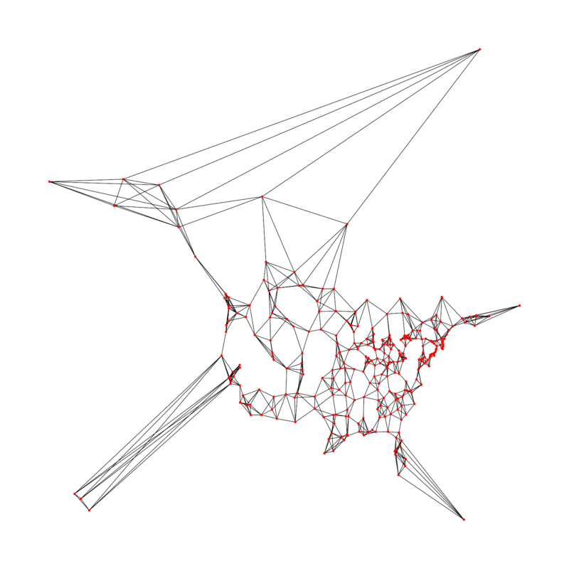
The graph consists of 312 North American cities. The edges represent cities’ nearest neighbours by distance. It is derived from the USCA312 dataset (local copy), which includes the entire distance matrix between cities. I pulled the five nearest neighbours of each city from this as edges to make an interesting graph. (Some cities participate in more than five edges, because a city might be in another city’s closest five cities even though the other city is not in its own closest five.) The edges are undirected.

Each city has x & y coordinates representing its geographic location (derived from the latitude and longitude). These are used to plot the graph.

The file city-graph.txt serializes the graph. Each non-indented line describes a city, giving its

• name,
• province (that is, state or province),
• x & y geographic coordinates of the city,
• the number of following indented lines that list (some of) its neighbouring cities
• (the “edges” it participates in), and
• the number of neighbouring cities (“edges”) for the city in total.

The indented lines following a city line gives

• the name & province of the neighbouring city, and
• the distance in miles (sorry!) to that neighbouring city. (You will not be using this information in this project. We only care whether there is an edge between two cities or not.)

Only neighbouring cities that have appeared earlier in the file are listed under each city line. Since edges are undirected in this graph, this is adequate.

Find the “original” USCA312 dataset at GitHub. Thanks to John Burkardt presently at the University of Pittburgh, previously at Florida State University, who further curated the USCA312 dataset (FSU copy).

The Algorithm

The objective is to remove edges based on edge betweenness with respect to the graph to break the graph into two connnected components; thus, to identify two “communities” of North American cities. Do this by the following algorithm.

• Repeatedly remove the edge with the largest betweenness score until the graph is disconnected.
• After each edge removal, recompute the remaining edges’ betweenness scores — that is, with respect to the “new” graph that resulted from the previous edge removal — since the edges’ betweenness scores may now have changed.
• Once the graph has become disconnected, add back as many edges to the graph that you had deleted as possible that still leaves the graph disconnected. (Note that this is simply adding back each deleted edge that is between nodes in one or the other connected component, but that is not a “bridge” edges between the two components.)

When I ran this on the city graph, my program removed 20 edges, then returned 9, leaving a twelve-edge cut of the graph. Note that a plot of the “cut” graph might not readily show a clear two regions with no lines between them; that also depends on how the graph is plotted with node position information. In this case, however, the separation is visually apparent.

Use the city’s name plus province as a unique label for its graph node; a city’s name by itself is not unique in the dataset.

The Algorithm

Use the Apriori algorithm for frequent itemset mining to find frequent itemsets that are synonomous with complete bipartite subgraphs in the graph, as discussed in class. These then represent “clubs”, small communities in the graph.

Task: Find the frequent itemsets of size three with a support count of four or more. A frequent itemset (right) paired with the “label” items of the transactions that support it (left) then constitutes a complete bipartite subgraph.

Or: Find the frequent itemsets of size eleven with a support count of 57 or more. (People are finding that the file of frequent itemsets of size three with a support count of four to be large; it is around five gigabytes.)

Thus, you are finding K≥4,3 or K≥57,11 to detect “clubs” of size at least 7 or of at least 68, respectively. Of course, your program should not be hardwired for these specific values.

Name your program cbs.py. It should take command-line arguments of

• level_of_frequent_itemsets: a file containing the frequent itemsets of length k (e.g., three) with respect to some support threshold (e.g., four),
• labelled_transaction_file: a file containing the labelled transactions, one per line, and
• a support-count threshold: the size of the support, the left of the complete bipartite clique (e.g, four), which is understood to be equal to, or to exceed, the implicit support count for the level_of_frequent_itemsets.

And it outputs the complete bipartite subgraphs found, one per line.

We can borrow an implementation of Apriori from the Data Mining class: levelUp.py. Note that you can generate the frequent itemsets per level using this for any transaction dataset in the right format. It does not produce level 1, though, as it needs the input of the previous level. You would need to make a file of the frequent 1-itemsets by hand or by other means.

You are welcome to adapt existing code as part of the your work, as long as it is clear that the code you use allows for derivative use (e.g., creative commons) and you attribute the source. That includes my levelUp.py.

Data Preparation

The musae files are not in the format that we need. So we have data preparation to do … as always.

For the graph data, we have it available as pairs of node-ID’s (comma separated), edges, in musae_facebook_edges.csv.

We want to have a transaction per line; each transaction is the set of nodes (by their integer IDs) that each have an edge to a given node, the transaction’s “label”. So we can transform the edge file to obtain this. Let us put the label as the first integer on the line, then followed by the integer ID’s belonging to that transaction. Let us make this space separated, since that is what levelUp.py wants for input. We did this in class: musae-ltrans.txt.

To use levelUp.py to generate our frequent itemsets level by level, it needs the transactions but without those transaction labels. Your cbs.py will need it with the labels (i.e., musae-ltrans.txt). Well, that is just the same thing, but stripping off the leading integer per line: musae-trans.txt.

We need a starter file for Apriori that has the frequent 1-itemsets; that is, the frequent itemsets of size one. For format, this will be one node-ID “integer” per line in our file. Since this is a small dataset, we can have it be all the node-ID’s, which is essentially the 1-itemsets with support count of zero or greater. The Apriori algorithm can make frequent k-itemsets with respect to a support-count threshold of n using the frequent (k−1)-itemsets with respect to a support-count threshold of m, as long as m≤n (just maybe not as efficiently). And we should have the lines sorted, for convenience: musae-one-sc0.txt. Not a very interesting file, but there you go.

Now the set of 2-itemsets with respect to a support-count threshold of zero would be huge! it would be all pairs of nodes. So let’s not do that. Let’s generate it with a support-count threshold of four, to be more reasonable.

% python3 levelUp.py musae-one-sc0.txt musae-trans.txt 4 > musae-two-sc4.txt

Okay, that took my iMac ten minutes. It found 636,132 2-itemsets. But two is usually an expensive step for Apriori. Editing out the leading integer per line in the output file (which is the support count for the itemset), I got musae-two-sc4.txt.

And with a higher support count of 57:

% python3 levelUp-nsup.py musae-one-sc0.txt musae-trans.txt 57 > musae-k2-sc57.txt
% python3 levelUp-nsup.py musae-k3-sc57.txt musae-trans.txt 57 > musae-k4-sc57.txt
    ⋮
% python3 levelUp-nsup.py musae-k9-sc57.txt musae-trans.txt 57 > musae-k10-sc57.txt

Note that levelUp-nsup.py here is just levelUp.py with the parts to print the support counts and statistics edited out.

Here is what I obtained: musae-k10-sc57.txt.

Report for Clubs

The main deliverable for Q. Clubs is your program, cbs.py.

Identify a couple of clubs that you found in the graph. The file musae_facebook_target.csv maps the node integers used in the edge file to descriptions. Translate your found clubs into the descriptions.

Lastly, answer the question of whether clubs — a club is the set of nodes of a complete bipartite subgraph — can overlap or if they must be disjoint.