Description
ECE 269 Project Description
List of Projects
1. Sparse Dictionary Learning: In many signal processing problems, the objective is to represent a
signal as a linear combination of known vectors (also called atoms), and these atoms form a dictionary.
Let Φ ∈ CM×N be a dictionary and φi
, i = 1, 2, · · · , N are the atoms. We seek to represent a signal y
as a linear combination of these atoms, i.e find coefficients xi such that y =
PN
i=1 xiφi which essentially
requires us to find solution to the following system of linear equations:
y = Φx (1)
If the dictionary Φ is chosen to be overcomplete (N > M) containing a basis, it is possible to represent
any signal y ∈ CM. However, the system of linear equations (1) will have infinite number of solutions
in x. Thus, we need the notion of sparsity where the objective is to look for the sparsest x (i.e. x
with minimum number of non-zero elements) which satisfies (1). This amounts to solving the following
optimization problem:
min
x
||x||0 (2)
subject to y = Φx
1
Popular examples of the dictionary Φ are DFT, DCT or Wavelet dictionaries. The ability to obtain a sparse representation depends on the class of signals, as well as the choice of the dictionary.
This is the motivation to understand if it is possible to “learn” a dictionary given a certain class
of input signals. Let yi
, i = 1, · · · , k be training samples from which we want to learn the dictionary Φ such that it permits sparse representation for every yi with sparsity at most L. Let
X =
x1 x2 · · · xk
, Y =
y1 y2 · · · yk
. Dictionary learning can be cast as the following
optimization problem:
min
X,Φ
||Y − ΦX||F (3)
subject to ||xi
||0 ≤ L
In this project you are expected to do the following:
(a) Read the papers listed in the reference and reformulate the sparse representation problem when
noise is added to the signals.
(b) Discuss at least three commonly used techniques in Dictionary learning. State the assumptions
that are necessary for ensuring uniqueness of this problem. Is the decomposition Y = ΦX always
unique, or are there some trivial ambiguities ?
(c) Given a fixed dictionary, implement Orthogonal Matching Pursuit (OMP) to obtain a sparse
representation for any given signal. Is OMP always successful ? Show numerical examples.
(d) Implement k-SVD to generate adaptive dictionary using a training dataset of clean images. You
may want to try synthetic data first before using real data.
(e) One of the applications of signal representation using overcomplete dictionaries is de-noising. Add
Gaussian noise to a test image and obtain a sparse representation using the dictionary learned in
(d). Is the reconstructed image noisy ? Explain your observation. Compare the reconstruction
quality with fixed dictionary and adaptive dictionary. Show the effect of addition of noise at
different levels and different noise models (Gaussian, Poisson etc). Plot the dictionary that you
learned using k-SVD.
(f) (Bonus:) In practical applications, you may not have access to clean images and thus, you may
need to learn the dictionary from the corrupted data itself. Paper (iii) provides an algorithm to
achieve this by using k-SVD. Study and implement the algorithm.
References:
i M. Aharon, M. Elad, and A. M. Bruckstein. “On the uniqueness of overcomplete dictionaries,
and a practical way to retrieve them.” Linear algebra and its applications, vol. 416, no. 1,
pp.48-67,2006.
ii M. Aharon, M. Elad, and A. Bruckstein A. “k-SVD: An algorithm for designing overcomplete
dictionaries for sparse representation.” IEEE Transactions on signal processing, vol. 54, no. 11,
pp. 4311-22, 2006.
iii M. Elad, M. Aharon. “Image denoising via sparse and redundant representations over learned
dictionaries.” IEEE Transactions on Image processing, vol. 15, no. 12, pp. 3736-45, 2006.
iv D. P. Wipf, and B. D. Rao. “Sparse Bayesian learning for basis selection.” IEEE Transactions on
Signal processing, vol. 52, no. 8, pp.2153-2164, 2004.
v J. A. Tropp, and A. C. Gilbert, “Signal recovery from random measurements via orthogonal
matching pursuit.” IEEE Transactions on information theory, vol. 53, no. 12, pp. 4655-4666,2007.
vi Y. C. Pati, R. Rezaiifar, and P. S. Krishnaprasad. “Orthogonal matching pursuit: Recursive
function approximation with applications to wavelet decomposition.” In Conference Record of
The Twenty-Seventh Asilomar Conference on Signals, Systems and Computers. pp. 40-44. IEEE,
1993.
2
2. Recommender system using Matrix Factorization:
A recommender system tries to model the preference of a user by analyzing the usage pattern and
make appropriate suggestions. Recommendation systems have become ubiquitous in many areas such
as movies, music, e-commerce. The data for a recommendation system is often stored as a matrix
A ∈ RM×N where tM users provide ratings for N items. Matrix factorization models aim to decompose
this rating/preference matrix as a product of two matrices.
A = PQ, P ∈ RM×K, Q ∈ R
K×N
This factorization of the matrix allows us to map each user as well as each item to a common latent
space of dimension K ≤ min(M, N). The resulting dot product, p
T
i
qj , captures the interaction between
user-i and item j that will allow the recommender system to make predictions. In this project you are
expected to do the following:
(a) Read the papers listed in the reference and discuss different techniques used for designing a
recommendation system.
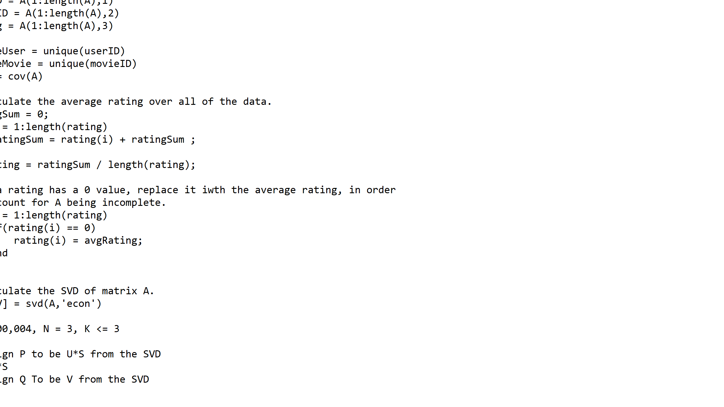
(b) Read (i) and (iii). Using real data, implement a recommendation system using the Singular Value
Decomposition (SVD) based technique. In most cases, the matrix A is incomplete. Can you
directly use SVD or do you need to make certain assumptions?
(c) Compare the performance of your implementation of (b) with alternative approaches given in (a).
Explain the performance evaluation metrics used.
(d) Does the implementation in (b) take care of new users/items ? Suggest a modification in (b) to
incorporate addition of new items (and users) with proper mathematical justification. Compare
the performance of this on-line system with the off-line version.
(e) (Bonus:) There are alternative ways to deal with the problem of incomplete data matrix. Reference (ii) provides two algorithms based on Stochastic Gradient Descent and Alternating Least
Squares. Study and implement these algorithms.
References:
i P. Cremonesi, Y. Koren, and R. Turrin. “Performance of recommender algorithms on top-n
recommendation tasks.” In Proceedings of the fourth ACM conference on Recommender systems,
pp. 39-46. ACM, 2010.
ii Y. Koren, R. Bell, and C. Volinsky. “Matrix factorization techniques for recommender systems.”
Computer vol. 42, no. 8 (2009).
iii B. Sarwar, G. Karypis, J. Konstan, and J. Riedl. “Application of dimensionality reduction in
recommender system-a case study”, innesota Univ Minneapolis Dept of Computer Science 2000.
iv B. Sarwar, G. Karypis, J. Konstan, and J. Riedl. “Incremental singular value decomposition algorithms for highly scalable recommender systems.” In Fifth International Conference on Computer
and Information Science, pp. 27-28. Citeseer, 2002.
v M. W. Berry, S. T. Dumais, and G. W. O’Brien. “Using linear algebra for intelligent information
retrieval.” SIAM review, vol.37, no. 4, pp. 573-595, 1995.
Dataset Suggestion: Jester (dimensions 24983 X 101)- https://www.ieor.berkeley.edu/ goldberg/jesterdata/
3. Robust Linear Regression
This paper studies a robust linear regression problem based on OMP.
3
(a) Read the entire paper carefully (including the appendix) and implement the original GARD
algorithm (see Algorithm 1 on page 4). The authors further use Cholesky decomposition to speed
up their algorithm. Try to use QR decomposition as well as Matrix Inversion Lemma instead of
Cholesky decomposition for faster implementation.
(b) Compare GARD (one of your fast implementations) with least squares and M-estimators (see
MATLAB robustfit function, and choose any two weight functions) by conducting the experiments
described in section V.A, V.C, V.D of the paper (no need to compare with other methods listed
in the paper).
(c) In experiment section V.A, compare the run-time of all versions of GARD (original, QR, Matrix Inversion Lemma) with least squares and M-estimators. Finally, test these methods on any two real
datasets given below: https://people.sc.fsu.edu/ jburkardt/datasets/regression/regression.html (x01.txtx28.txt) E.g., The selling price of houses is to be represented as a function of 11 variables:
https://people.sc.fsu.edu/ jburkardt/datasets/regression/x26.txt
References:
i G. Papageorgiou, P. Bouboulis, S. Theodoridis, and K. Themelis, “Robust linear regression analysis – a greedy approach.” IEEE Transactions on Signal Processing vol. 63,pp. 3872-3887, 2015.
4. Transceiver Design via Generalized Triangular Decomposition (GTD)
These two papers introduce the idea of Generalized Triangular Decomposition (GTD) that provides the
most general unitary decomposition of a complex matrix. Several known decompositions such as the
Singular Value Decomposition (SVD) and the QR Decomposition become special cases of GTD. Reference (2) establishes the mathematical foundations of GTD (such as its existence) and algorithms for
computing GTD, whereas reference (1) shows how GTD plays a central role in transceiver optimization
for MIMO channels. In this project, you will
(a) Implement the GTD algorithm and use the GMD decomposition for transceiver design with the
zero-forcing VBLAST (ZF-VBLAST) detector, following the method described in Sec IV and V
of reference (1).
(b) Produce the BER plots similar to Fig 3, 4, 5 in reference (1).
(c) Test your code and verify that SVD and QR decomposition are special cases of GTD. Note:
Although reference (2) contains MATLAB codes for GTD, you should not use it, but develop
your own MATLAB code for implementing GTD.
i Y. Jiang, J. Li, W.W. Hager. “Joint transceiver design for MIMO communications using geometric
mean decomposition.” IEEE Transactions on Signal Processing, vol. 53, pp. 3791-3803, 2005.
ii Y. Jiang, W. Hager, J. Li. “The generalized triangular decomposition.” Mathematics of computation vol. 77, pp. 1037-1056, , 2008.
4


