Description

Overview

 

 

Our last assignment had us produce wireframe images of a 3-D scene using a form of ray casting. In this assignment we write code that renders using ray tracing. This is a more straightforward method for rendering of a scene by casting rays. Taken to its fullest level of detailing, the technique can be used to create extremely realistic images of a virtual scene. We model light transport, accounting for how light energy interacts with material, and we (in essence) follow light from their sources into the scene, see how they reflect off objects, and (perhaps) eventually hit the eye of the viewer so that they see those objects.

To make this feasible, ray tracing performs this “light following” in reverse: we trace rays from the eye out to the scene, see what objects are hit by that ray, and then see how light illuminates them. We do the latter— seeing whether and how the light illuminates objects— by tracing rays from the objects we hit. If an object is a mirror, we trace a ray in the direction of reflection to find out what object can be viewed in that mirror’s image. With enough of this kind of tracing, enough realistic modeling of surfaces and how materials behave, and enough computational resources, ray tracing and its variants are the basis for most photorealistic CG-rendered animated movies today.

The code for this project performs ray tracing using the graphics hardware. We will write the ray tracer within the code of a fragment shader in the C-like language GLSL. This is somewhat unusual, as ray tracing is typically performed off-line. It is the same kind of code we’ve used to support our rendering in past projects, but those shaders implemented the standard z-buffer based graphics pipeline, using an approach that is much different than ray tracing.

For the assignment, you will extend some existing ray tracing GLSL code so that it handles a mirrored surface described by a quadratic Bezier curve. The code you are given ray traces spherical and planar objects, using Phong shading, and also for spherical mirrors. Your job is to extend the scene editor and the ray tracer to handle scenes with a curved mirror.

As a consequence of ray tracing in the hardware, the scene can be edited in a web application written in Javascript, and the updated rendering can be viewed in real time. The calculations would normally be too expensive to perform in Javascript, but a GPU can instead quickly trace the 512 × 512 × 4 rays used to depict the scene. Even so, we keep the scene and simple to make this feasible. More general ray tracing would bog down the GPU too much,

Starting code and assignment

Here is the starter code for this assignment. If you download this code, you’ll will find three important code source files:

 

• bezier-funhouse.js: this code is the main driver for the javascript/WebGL application. It contains a scene editor that allows its user to place spheres and to edit the shape of the mirror. It then calls the GLSL code to ray trace and render the scene. 

   

• funhouse.js: this defines two classes Sphere and Curve for the two scene object types. They can be positioned in the scene, and their info gets passed to the ray tracer. 

   

• bezier-funhouse.html: the top of this file contains the GLSL source code for trace-vs.c and trace-fs.c. They work together to perform ray tracing of the scene in the hardware.

 

For the asignment you will modify funhouse.js and trace-fs.c so that they properly handle the funhouse mirror whose footprint is specified as a quadratic Bézier curve.

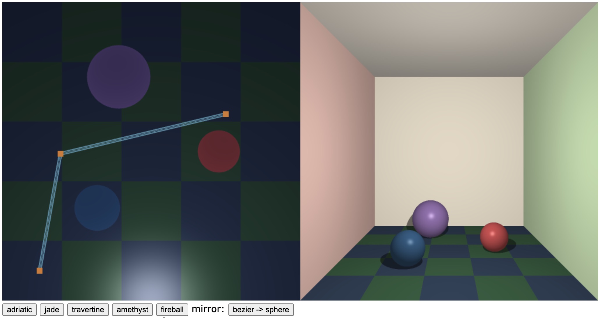
To run the code, load bezier-funhouse.html into your browser. With its initial settings it allows the user to create a scene full of spheres. It also displays a spherical mirror, one that can also be resized and moved. Figure 1 shows an example of a scene where five colored spheres have been placed around that mirror ball. The left view shows the scene from above, and uses the algorithms described last week to display the layout on the floor of the room. The right view shows the ray-traced scene produced by the shader code.

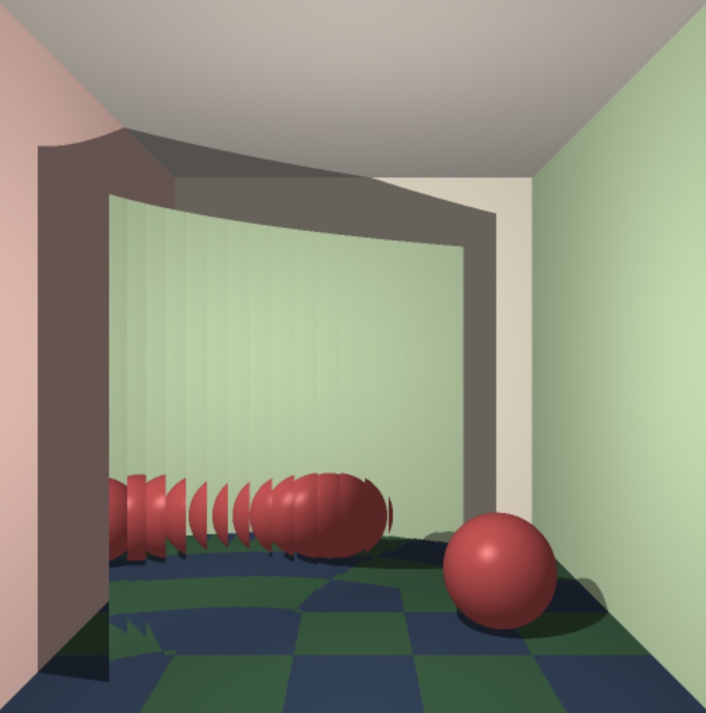
Figure 2 shows the results you can obtain once you’ve completed the assignment. When the application is switched to display the Bezier funhouse mirror, the scene editor shows the control points for the footprint (the top view) of a curve. And the ray tracer shows a picture with some scene objects warped and reflected in that funhouse mirror. It also depicts the shadow of that mirror falling on the back part of the room.

The Assignment

 

Figure 3. The initial program in Bezier mode. Left: the editor poorly approximates the curved mirror. Right: the renderer ignores the mirror’s existence.

 

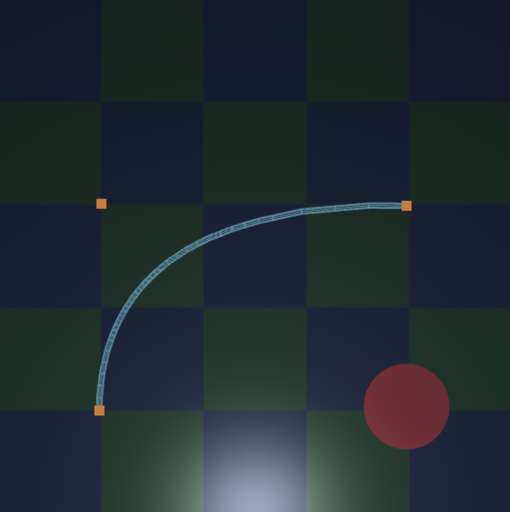
In its current state, if you click on mirror:sphere -> bezier and switch the application from displaying the spherical mirror, to allow edit and display of the funhouse mirror, you’ll see very little of that functionality. This state is shown in Figure 3. On the left, you’ll see that the editor uses the control polygon as the points of the quadratic Bezier curve. This is obviously a problem. The editor should instead show a smooth curve running from the first control point to the third, and using the second control point to suggest the curvature of the mirror.

 

• Change the editor to display a Bezier curve for the three control points.

 

To complete this step, you’ll need to modify the compile method of class Curve so that it computes an array of curve points. It should sample enough points on the curve to produce that array, and its method for doing that should rely on SMOOTHNESS. Larger values lead to a smoother approximation. It should lead compile to use more points. The sampling ideally should depend on the curvature of the Bezier. A flatter curve should use fewer points. A more pronounced curve should require more.

You’ll notice also that ray-traced view shows nothing initially when placed in Bezier mode.

 

• Change the ray tracer to display a Bezier funhouse mirror that reflects the objects and walls of the scene.

 

This coding involves writing two key functions in trace-fs.c within bezier-funhouse.html. The first, rayIntersectsBezier is used by rayIntersectsMirror to handle computing a ray of reflection when a traced ray hits the funhouse mirror. You can use a similar subdvision technique to compute the mirror’s geometry that you did for the editor, however the normal that you compute that aids in determining the reflection ray should be smoothly interpolated so that there are no obvious discontinuities of the scene in the mirror.

 

• Smoothly interpolate the normal of the mirror over its surface.

 

The second key GLSL function you need to write is rayHitsBezierBefore. This is used to figure out whether an object in the scene is in the shadow of the funhouse mirror. When the ray tracer hits a wall or a non-reflective sphere, it computes Phong shading of that surface by tracing a ray from the object to the light source. If the mirror sits between that surface point and the point light source, then it casts a dark shadow on that object and it won’t reflect anything but the ambient light of the room. The Phong shader uses rayHitsBezierBefore to check for that shadow.

 

• Change the ray tracer to display the shadow of the Bezier funhouse mirror.

 

To guide you through completing the assignment, we first walk you through the current ray tracing code just below. And then we briefly describe our methods from class for sampling points on a Bezier curve. Finally, we walk you through a plan for completing the assignment.

Raytracing the funhouse

Let’s talk a bit about the state of the inital code and how the edited scene becomes the ray-traced funhouse image.

The funhouse room with Phong shading

The initial code has a simple ray tracer that handles a 4-walled room. There is one point light source initially sitting above the entrance to the room. The room has four walls and a checkered floor. A user can place spheres of different sizes onto the floor of the room. And then also the code handles computing the reflections within a single mirrored object.

Non-mirror surfaces are rendered using Phong shading. The walls, ceiling, and floor are treated as matte surfaces of different-colored materials. This means that they have an ambient and diffuse (Lambertian) component that they reflect when illuminated by a point light source. If a wall is in shadow from the light, then only the ambient light of the room is reflected.

The non-mirror spheres sitting in the room are treated as glossy surfaces, again using the Phong model. If they are in shadow, they reflect only ambient light. If they are directly illuminated by the light, then there are also difuse and specular components to their reflected light. This means that they have a small specular highlight placed with the peak of the highlight at the perfect mirroring direction for the light source.

This calculation for spheres and walls is just the local illumination model we covered several weeks ago in class when describing classical hardware rendering. It is summarized by the pseudo-code below.

PHONG-COMPUTE-COLOR(P, n, V, L, m):
   a := ambient from m.color at P
   d := diffuse from m.color because of n wrt L at P
   s := highlight at P because of n wrt L viewed from V
   hits-light := SHOOT-RAY(P, L-P) // shadow ray
   if hits-light:
      return a + d + s
   else:
      return a

In the code P is the point on the surface being illuminated, n is the surface normal, V is the point from which we are viewing the object, L is the location of the (single) light source, and m stands for the material’s properties.

We have one enhancement in the Phong shading code: We don’t assume that P is directly illuminated by the light. Instead we shoot a ray out from P towards L to see if any scene objects get in the way of the light. If they do, hits-light returns false and we only give back the ambient component. If instead the light is hit by the “shadow ray”, then we also include the diffusely reflected light, possibly along with some glossy highlight.

So, already, we’ve tweaked direct illumination so that it traces a shadow ray to create a more realistic rendering. Objects cast shadows on other objects in the scene.

For mirrored surfaces, when a point on the mirror is visible, then we figure out the color of light reflected off the mirror from some other (non-mirror) object, or else the walls, ceilings, and floors in the room.

This is described in more detail below.

Raytracing the scene

For our ray casting algorithm for Program 3, we shot rays through a virtual screen representing a piece of paper to see where each corner of an object’s mesh would fall on the page. We then judiciously connected those dots to build a wireframe rendering of the objects in the scene.

Ray tracing has a similar set up. We choose a point outside the scene as a center of projection. And then we place the pixels of a virtual screen in front of that point, with the pixels forming a regular grid. That grid of pixels acts as a window into our virtual 3-D scene of objects. And then, with ray tracing, we shoot rays for each one of those pixels. The goal of these rays is to trace backwards from the eye (from the center of projection) through each pixel into the 3-D scene to determine what object is reflecting light, and at what color, towards our eye’s view. This top-level ray tracing algorithm is summarized below:

RAY-TRACE-SCENE():
   R := center of projection; source of primary rays
   for each pixel x of the virtual screen's grid:
      d := direction from R through x
      c := TRACE-RAY(R,d) // primary ray
      paint x the color c

In the above, we use R as the source of the ray, and d as the direction it is shot through some pixel location x. We obtain information about the scene by a call to TRACE-RAY. This checks the world to see what object is providing a color c of light hitting us from the scene.

By tracing backward this “primary ray”, we can make standard geometric calculations— “Is this sphere visible first along this ray?”— to ask questions about the scene, figuring out how light is illuminating our scene. Each ray serves to query the geometry of the scene. If we hit an object with our query ray, we’ll then typically shoot “secondary rays”. With those secondary rays we ask questions like “Does this object have a direct line of sight to a light source?” and “Is this object a mirror? What light then does it reflect?”

This is summarized by the pseudocode below. The ray we trace might hit a wall, or a sphere, or the mirror. For non-mirror objects we use our modified PHONG-COMPUTE-COLOR that includes shadow ray tests to determine the color of that object.

TRACE-RAY(R, d):
   shoot a ray from R in direction d
   if a wall is hit at point P with normal n:
      L := position of the light
      c := PHONG-COMPUTE-COLOR(P, n, R, L, material hit)
   if instead a sphere is hit first at point P with normal n:
      ... do the same PHONG computation...
   if instead the we hit the mirror at point P with normal n:
      r := the reflected ray direction
      c := TRACE-RAY'(P, r) // secondary ray
   return the color c

When instead a mirrored object is hit, that leads us to bounce a secondary, reflected ray to find out the color of light that’s hitting the mirror and bouncing towards our eye. In general ray tracing, this normally leads to a recursive call to TRACE-RAY. For this assignment, in order to make hardware ray tracing feasible, our secondary ray ignores mirrored objects. Thus we call a TRACE-RAY' that behaves almost the same, but skips the mirror check.

That’s pretty much it. But this pseudocode doesn’t quite give a complete enough picture of the assignment. Let’s now discuss the vertex and fragment shaders we’ve written in GLSL. These essentially mimic the pseudocode above, but their details will be useful to know.

Raytracing in GLSL

The key file that implements the ray tracing is the code for trace-fs.c. That code is invoked once for each pixel on the WebGL canvas, running something like the following code:

void main(void) {
    vec4 rayDirection = intoDirection
                      + (ray_offset.x + dx) * rightDirection
                      + (ray_offset.y + dy) * upDirection;
    vec3 color = trace(eyePosition, rayDirection);
    gl_FragColor = vec4(color, 1.0);
}

The code is sent eyePosition, into, right, and up. These are uniform, meaning every pixel gets sent the same info for these. In addition, every pixel is sent an xy pair ray_offset with coordinates taken from [−1,1]×[−1,1][−1,1]×[−1,1]. These have us shoot each primary ray through a particular location in the screen.

Most of the rendering work is done within trace. This code for this function starts roughly as follows:

ISect mirror    = rayIntersectMirror(R,d);
vec4  source    = R;
vec4  direction = d;

if (mirror.yes == 1) {
    bool blocked = rayHitsSomeSphereBefore(mirror.location, -d, FAR);
    if (!blocked) {
        source    = mirror.location;
        vec4 n    = normalize(mirror.normal);
        direction = normalize(d - 2.0 * dot(d,n) * n);
    }
}

...

We shoot the primary ray defined by R and d to find whether it intersects with the mirror, using rayIntersectMirror. We then see if there is any intervening sphere by calling rayHitsSomeSphereBefore. The goal of this is to determine a source and direction to compute the Phong illumination of some object or wall in the scene. If the mirror isn’t hit by the primary ray, we just directly look for an object or a wall by setting source to R and direction to d. If instead there is a mirror bounce, then we set source and direction to the mirror intersection and the bounced reflection ray instead.

Here is the remaining code for trace:

...

ISect sphere = rayClosestSphere(source, direction);
ISect wall   = rayClosestWall(source, direction);
ISect isect  = bestISect(wall,sphere);

color = computePhong(isect.location, isect.normal,
                     source, lightPosition,
                     isect.materialColor,
                     isect.materialGlossy);
}

return color;

Again: that’s all there is to it. This isn’t quite the pseudocode we gave earlier but it is similar.

Intersection struct

The code above relies on a GLSL struct for recording and reporting intersection information. For example, our mirror check, sphere check, and wall check each return this structure. Here is its definition:

If a traced ray fails to hit an object, then our code returns NO_INTERSECTION(). This is an ISect whose yes component is set to 0. If instead an object is hit, then yes is set to 1, and the next three components should hold the distance along the ray where it hit, the point where the ray hits, and the normal to the surface where it was hit. The latter two are each a struct of type vec4, a structure with xyzw components, with w of 1.0 for a point and of 0.0 for a vector. The last two components give the RGB of the material’s color, and a 0/1 value indicating whether the material is matte or glossy.

We also regularly use the function bestISect which compairs two intersections, picking the closest valid one. Here is its code:

ISect bestISect(ISect info1, ISect info2) {
    if (info2.yes == 1 
        && (info1.yes == 0
            || info2.distance < info1.distance)) {
              return info2;
          } else {
              return info1;
          }
      }
}

If two object intersections are valid (their yes is 1) then we return the closer intersection. When we shoot a ray into the scene, this is our way of choosing the closest intersection— the first object we hit.

Tracing to a plane

I hope you are getting a sense of the nature of GLSL coding. In most cases we are working with integer, boolean, and floating point variables of type int, bool, and float. Like normal C coding, we introduce these variables with their type. And then we typically also work with 2-D, 3-D, and 4-D floating point vectors corresponding to the types vec2, vec3, and vec4. These are richly supported in GLSL. They have operations like + and *, and dot and cross, and normalize and length. I summarize these in an appendix below.

To illustrate some of this coding. let’s examine the code that is used to trace a ray to a wall, given below:

ISect rayIntersectPlane(vec4 R, vec4 d, vec4 P, vec4 n) {
    vec4 du = normalize(d);
    float height = dot(R - P, n);
    if (height < EPSILON) {
        return NO_INTERSECTION();
    }

    float hits = dot(-du, n);
    if (hits < EPSILON) {
        return NO_INTERSECTION();
    }

    float distance = (height / hits);

    ISect isect;
    isect.yes      = 1;
    isect.distance = distance;
    isect.location = R + distance * du;
    isect.normal   = n;
    return isect;
}

We first normalize the ray’s direction as du, then project the line from R to P onto the plane’s normal to compute the ray source’s height away from the plane, making sure that it is on the correct side of the plane. And then we see whether the ray direction lines up in opposition to the surface normal. If all that works out, we record all the intersection information and return it.

For your coding, you will want to write the same kind of code, but for the Bezier funhouse mirror. There is also similar code for ray-sphere intersection, It’s worth checking this code out, too, under the function named rayIntersectSphere.

Scene and Editor Coordinate Systems

Once again we have a coding project that juggles a few coordinate systems to do its work. There are the points in the scene. Within the scene editor, these are represented as Point3d objects. Their xyz coordinates are within the range [−1,1]×[0,2]×[0,2][−1,1]×[0,2]×[0,2]. When looking at the editor, we are getting a top view and points with x=0x=0 and z=0z=0 sit at the middle of the bottom. This corresponds to the front of the room. Moving spheres left and right within that editor view decreases and increases their xx coordinate, and also moves them left and right in the room. Moving them forward and backward pushes them away, and then moves them closer to the front of the room. This increases and decreases their z coordinate. Items sit on the floor at the plane y=0y=0. The tops of spheres have more positive yy values than lower parts of the spheres.

Note that this means that the scene coordinates are interpreted in a left-handed coordinate system. The xx axis points right in the rendered view of the room, and the yy axis points upward. And then our view of the scene is in the positive zz direction.

The center of projection for the ray tracer is a point that sits at (0,1,−1)(0,1,−1). It is within the middle of the entrance square, but sits one unit behind it. We shoot rays from that point to each point on the square entrance wall to make our traced scene.

Lastly, the curve points for the funhouse mirror are sent to the shaders as 2-D coordinates. These have components xy but actually correspond to the xx and zz coordinates of the points on the base of the mirror (with y=0y=0 because the base sits on the floor). Consider the image of the editor below:

 

Figure 4. The editor showing a curve placement.

 

In the scene, we have the two curve control points on the left with their x=−0.8x=−0.8. The other control point is at x=0.8x=0.8. The top two control points are at z=1.2z=1.2. The lower point’s z=0.4z=0.4. So, in the editor code the top left point sits at Point3d(-0.8,0.0,1.2). But then these are passed to the GLSL shader code as vec2(-0.8,1.2).

Another Walk Through

Here I give you a plan for completing the assignment. Most of the technical work relies on your continuing application of vector and affine calculations, and also some of the key details we emphasized about Bezier curves. I won’t review those here, instead I offer an approach that fits the bill, references some of that material, and orients you to the places you’ll do your coding.

I should first note that there are technically only three places that require your changes. You can find them by grep-ping for COMPLETE THIS CODE in the Javascript, and CHANGE THIS CODE in the HTML/GLSL.

Step 1: Compiling the Editor Curve

As an immediate warm-up to your task, I recommend getting the editor to display a curve for the given control points when in Bezier mode. You need to modify the compile method of Curve so that it creates a list of Point3d objects that are a smooth-enough set of samples of the Bezier curve. These should have their xz coordinates vary, and should sit on the floor with y=0y=0, just like the control points.

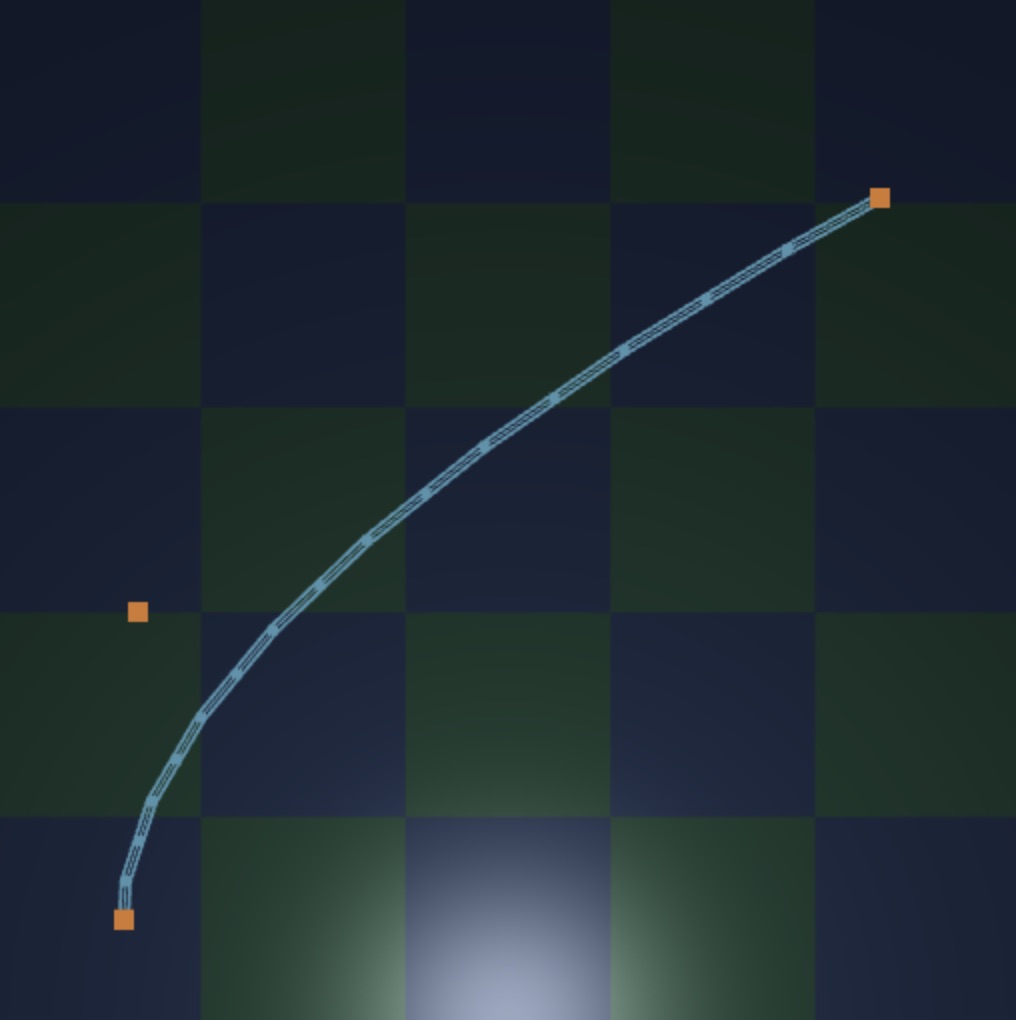
One way to get this working is to just evaluate the polynomials with a regular sampling of the parameter interval from 0.0 to 1.0. Figure 5 shows a regularly spaced rendering performed this way, and with only 17 points just to illustrate the idea.

 

This is fine for a start, but I’d ultimately rather have you use this exercise as a way of learning deCasteljau’s subdivision scheme. This is naturally recursive. Each attempt to compile a curve with control points P0P0, P1P1, P2P2 relies on two recursive calls to evaluate “left” and “right” curves with, say, control points L0L0, L1L1, L2L2 and R0R0, R1R1, R2R2. I’ll leave you to your notes to remind yourself of the formulation.

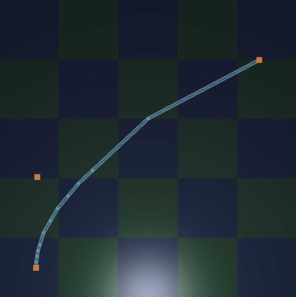
This strategy requires a base case. In my solution, I use the 1.0/SMOOTHNESS as an “epsilon tolerance” for the two sides P0P1P0P1 of the polyline P1P2P1P2 to be close enough to approximating their underlying curve. Figure 6 shows an adaptive rendering performed this way, and with a low SMOOTHNESS (high tolerance) just to emphasize the approach.

 

Having set this.points with enough, and appropriate, samples, the editor should display the curve.

Step 2: Ray Tracing a Polygonal Mirror

The next thing you must do is write the code for rayIntersectMirror in the GLSL ray tracer so that it displays a funhouse mirror. It is written to rely on the function with the C prototype:

ISect rayIntersectBezier(vec4 R, vec4 d, vec2 cp0, vec2 cp1, vec2 cp2);

It assumes a tall Bezier-shaped mirror is specified by “floor coordinates” suggested by the 2-D coordinates of control points cp0, cp1, and cp2. It should return a struct of type ISect that describes intersection of the ray with that mirror.

My approach to this had me approximate the mirror with a series of planar panels, regularly-spaced (in terms of the curve parameter) around the curve. Using this approach I built a helper function rayIntersectPanel that performs ray-panel intersection for a floor-standing mirror with whose fotpriont is a line segment. This rerlied on rayIntersectPlane provided in the code.

You can try out this code by just displaying the polyline-bottomed mirror of the curve control points. This will be satisfying to get working first, and you can test it by moving the mirror around.

This isn’t quite what we want. We’d like a smoother approximation of the geometry of the curve. And we’d like no discontinuities in the reflection in the mirror. To tackle the latter concern, my code performs a smooth interpolation between two normals: one for the left side of the panel, one for the right side of the panel. That interpolation is an affine one. The combination weight can be calculated based on the position of the intersection with the panel. Figure 7 shows my solution before adding interpolating the normal vector.

To get smoothness in the geometry you can subdivide a fixed number of times. This “fixed number” is necessary because of the limits of GLSL. It is not possible to write recursive code in GLSL, and it is not possible to write indefinite loops. The shader compiler needs to know that the code will terminate when run on the GPU, and so it limits the kinds of programming we do.

 

For my solution I wrote a recBezier1, a recBezier2, etc. to handle the different depths of the recursion.

Step 3: Shadows

If you complete Step 2 in some way, you won’t see any shadows. This is because the ray tracing code relies on a different function

bool rayHitsBezierBefore(vec4 R, vec4 d, vec2 cp0, vec2 cp1, vec2 cp2, float distance);

The spec for this function is similar to rayIntersectsBezier, but it instead returns true or false, returning true when there is a ray-mirror intersection. This code is called by the Phong shading function to check whether a surface point is occluded by some intervening object between the light and the object. And so the code needs to check whether the mirror blocks the light between its location and the surface point that may be in shadow.

The distance value should be checked to see if, when the mirror is intersected by the given ray, it is intersected within a certain distance along the ray.

This code can just be a modification of your approaches in Step 2, refigured for a bool type and for a distance.

Step 4: Raytracing the Funhouse Mirror

Lastly, just do the work of Step 2 and Step 3 so that they give a smooth-enough approximation to the curved mirror. If you interpolate the normals as suggested, then you’ll find that a subdivision into 16 or 32 panels is good enough.

Congrats! You are done. Check out some bells and whistles below, or devise your own.

Summary and Hand-In

Thge steps above are probably the best way to approach completion of the assignment. You’ll get a taste for computing with Bezier curves in Javascript by completing the first step. You’ll get a taste for GLSL ray tracing with the second, followed by an easy change with the third. The fourth step is the main assignment, and hopefully you’ll have had enough practice with GLSL to tackle it. Step 4 is mostly just the marrying of ideas from Step 1 with the coding of Steps 2 and 3.

In summary:

 

• Write Curve.compile so that it computes the sample points of a Bezier curve at an appropriate level of detail, as specified by SMOOTHNESS. For a Curve instance this, it does this by building the array this.points. 

   

• Write the GLSL code for rayIntersectPanel and rayHitsPanelBefore so that the ray tracer renders the reflections and shadow of one pane of a polygonal mirror. 

   

• Write the GLSL code for rayIntersectBezier and rayHitsBezierBefore so that the ray tracer renders the reflections and shadow of a curved funhouse mirror. It can use a 5-level subdivision, treating the mirror as a 32-sided polyline, but then should smoothly interpolate the surface normal to obtain a funhouse reflection.

 

 

 

Bells and whistles

 

• softer shadows.

 

Change the code so that the light source isn’t a point light source. This would require you to hit several rays to a light to compute softer shadows. Alternatively, you could compute penumbra.

 

• multiple mirror bounces.

 

Our code doesn’t look for mirror hits when tracing a secondary ray. This means that a curved mirror cannot be seen as its own reflection. You can rewrite the code so that it shoots tertiary, etc. rays, if a bounced ray would hit a mirror. Similarly, you could allow the editor to place multiple spherical mirrors, or else a mix of sphere and funhouse mirrors.

 

• caustics.

 

We could check whether a point on the wall or a sphere is hit indirectly by light bouncing off the mirror.

 

• bi-quadratic mirrors.

 

Our funhouse mirror can be thought of as a bi-quadratic bezier patch, but where the 9 control points come in three sets of co-linear control points. You could generalize the mirror to instead be an arbitrary patch, figuring out a way to have all nine control points editable. And then also figure out the mirror calculatons. Note that a deCasteljau subdivision can easily be built for Bezier patches, so you can write the ray-patch intersection code using a similar method to our funhouse intersection.

 

• animate the scene.

 

You could add “physics” to the scene so that the spheres bounce around, or the mirror moves. This would update in real time, and would be no more expensive to render than a static scene.

 

• fly through.

 

Change the code so that the viewpoint and view direction moves, making the scene something that’s flown through. In order to deal with walls, you might change the scale of the ray trace, making the virtual screen smaller, and also making the view frustum smaller (putting the center of projection closer to the screen).

 

• stochastic ray tracing.

 

We approximate the reflection of spheres using Phong shading. We could instead, for example, shoot secondary rays from glossy objects. If we shoot several reflective rays from a sphere, we can get several samples of light that’s hitting the surface

 

• imperfect reflective funhouse mirror.

 

Building from the above suggestion, we could have a curved mirror that isn’t a perfect mirror. Instead, for example, it could diffusely reflect a color by collecting samples of light from several reflected directions using stochastic ray tracing.

Appendix: GLSL mathematics

The three kinds of vector structs used in GLSL are vec2, vec3, and vec4. Each have components of type float. Their components can be selected with xy, with xyz, and with xyzw. The vec3 type is also used for RGB colors. In actuality, GLSL often uses vec4 for colors, including the additional “alpha” component for transparency. Our code uses vec3 for RGB color values.

We build vectors with their constructors. There is some flexibility in doing so. For example, u = vec3(1.0,0.0,0.0); sets u to be the unit vector in the x direction. To make it include a w component, we can use v = vec4(u,0.0) to create it as vector v.

We can use the operations * and / to scale vectors v by a scalar a, for example, with the expressions v * a and v / a. You can add vectors componentwise with u + v. You can compute vector’s dot product with dot(u,v), which returns a float. You can also compute cross(u,v), but this is only defined if both u and v are of type vec3.

We can normalize(u) to compute a vector whose direction is the same as u but with unit length. You can get the length of a vector with length(u).

Many standard mathematical functions are defined on the float type, including abs, max, pow, sqrt, sin, and cos.